
Time series analysis is an essential skill when working with data that has a temporal component. Pandas provides a powerful suite of tools for analyzing and manipulating time series data, making it a go-to library for data analysts and data scientists. In this tutorial, we will cover the basics of working with dates and time in Pandas, as well as more advanced time series-specific functions.
Converting Date Strings to Datetime Objects
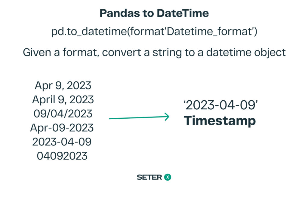
Before diving into time series analysis, it’s crucial to ensure that the dates in your dataset are represented as datetime objects. Pandas provides the to_datetime() function for converting date strings to datetime objects.
Let’s start by creating a DataFrame with date strings:
import pandas as pd

data = {
    'date': ['2021-01-01', '2021-01-02', '2021-01-03', '2021-01-04', '2021-01-05'],
    'value': [1, 3, 5, 7, 9]
}

df = pd.DataFrame(data)
print(df)
date value 0 2021-01-01 1 1 2021-01-02 3 2 2021-01-03 5 3 2021-01-04 7 4 2021-01-05 9
Now, let’s convert the date strings in the ‘date’ column to datetime objects:
df['date'] = pd.to_datetime(df['date'])
print(df)
date value 0 2021-01-01 1 1 2021-01-02 3 2 2021-01-03 5 3 2021-01-04 7 4 2021-01-05 9
You can also specify a format for the date strings if they are not in the default ISO 8601 format (YYYY-MM-DD):
df['date'] = pd.to_datetime(df['date'], format='%Y-%m-%d')
print(df)
By converting the date strings to datetime objects, you can now perform various time series-specific operations on your data.
Time Series-Specific Functions
Pandas provides a wide range of functions specifically designed for time series analysis. In this section, we’ll explore some of the most commonly used time series functions in Pandas.
Setting a Datetime Index
When working with time series data, it’s often beneficial to set the DataFrame index to be the datetime column. This enables you to efficiently perform various time series operations, such as slicing, resampling, and rolling windows.
To set the index to the ‘date’ column, you can use the set_index() method:
df.set_index('date', inplace=True)
print(df)
value date 2021-01-01 1 2021-01-02 3 2021-01-03 5 2021-01-04 7 2021-01-05 9
Time Series Slicing
With a datetime index, you can easily slice your time series data based on specific date ranges. For example, let’s select the rows in our DataFrame that correspond to the first three days of January 2021:
january_slice = df['2021-01-01':'2021-01-03']
print(january_slice)
value date 2021-01-01 1 2021-01-02 3 2021-01-03 5
You can also use partial strings to slice the data (but this way is deprecated). For instance, if you want to select all rows in January 2021, you can do the following:
january_data = df['2021-01']
print(january_data)
Resampling
Resampling is a technique used to change the frequency of your time series data, either by aggregating the data to a lower frequency (downsampling) or interpolating the data to a higher frequency (upsampling). Pandas provides the resample() method for this purpose.
For example, let’s downsample our daily data to a weekly frequency, calculating the sum of the ‘value’ column for each week:
weekly_data = df.resample('W').sum()
print(weekly_data)
value date 2021-01-03 9 2021-01-10 16
To upsample our daily data to an hourly frequency, you can use the interpolate() method to fill the missing values:
hourly_data = df.resample('H').interpolate()
print(hourly_data)
value date 2021-01-01 00:00:00 1.000000 2021-01-01 01:00:00 1.083333 2021-01-01 02:00:00 1.166667 2021-01-01 03:00:00 1.250000 2021-01-01 04:00:00 1.333333 ... ... 2021-01-04 20:00:00 8.666667 2021-01-04 21:00:00 8.750000 2021-01-04 22:00:00 8.833333 2021-01-04 23:00:00 8.916667 2021-01-05 00:00:00 9.000000 [97 rows x 1 columns]
Rolling Windows
Rolling windows are used to apply a function to a moving window of data in a time series. This technique is often used for smoothing noisy data, calculating rolling statistics, or detecting trends and patterns.
To apply a rolling window to your time series data, you can use the rolling() method. For example, let’s calculate the rolling 3-day mean of our ‘value’ column:
rolling_mean = df['value'].rolling(window=3).mean()
print(rolling_mean)
date 2021-01-01 NaN 2021-01-02 NaN 2021-01-03 3.0 2021-01-04 5.0 2021-01-05 7.0 Name: value, dtype: float64
You can also apply custom functions to a rolling window using the apply() method:
def custom_function(window):
    return window.sum() / window.count()

custom_rolling = df['value'].rolling(window=3).apply(custom_function)
print(custom_rolling)
date 2021-01-01 NaN 2021-01-02 NaN 2021-01-03 3.0 2021-01-04 5.0 2021-01-05 7.0 Name: value, dtype: float64
Learn more about applying functions in our tutorial on Pandas data transformation.
Frequently asked questions
Conclusion
In this tutorial, we explored the basics of working with dates and time in Pandas, as well as more advanced time series-specific functions, such as slicing, resampling, and rolling windows. By mastering these techniques, you can effectively analyze and manipulate time series data using Pandas.
To further develop your Pandas skills, consider exploring related topics like data visualization with Pandas, optimizing Pandas performance, and grouping and aggregating data with Pandas.